After starting my studies about machine learning at the college, I have been talking with people about it since then and I've come to realize that people, even with more technical background, still think about machine learning algorithms as a black box. Therefore I wanted to write this post showing how to implement the first proposed neural network model called Perceptron from scratch using R programming language. I am going to walk you guys throughtout the whole process, take a look and see what is inside of this black box.
Perceptron Neural Network
Neural network is a concept inspired on brain, more specifically in its ability to learn how to execute tasks. Actually, it is an attempting to model the learning mechanism in an algebraic format in favor to create algorithms able to lear how to perform simple tasks. Learning mechanism is such a hard subject which has been studying for years without a full understanding, however some concepts were postulated to explain how learning occurs in the brain, the principal one is plasticity: modifying strength of synaptic connections between neurons, and creating new connections. In 1949, Donald Hebb first postulated how the strength of these sinapses gets adapted, he says that the changes in the strength of synaptic connections are proportional to the correlation in the firing of the two connecting neurons. Does it sounds hard to get it right? Let me clarify things here. He simply said that if two neurons consistently fire simultaneously, then any connection between them will change in strength, becoming stronger. For example, do you remember the first time that you ate pizza from a new place and you loved the flavors? It was so good, right? Well, in that moment a set of neurons in your brain were stimulated positively, because you got happy tasting that pizza's flavors from new place, since these neurons fired at same time, it probably were connected together or created a new connection. Eventually, when you hear about that place from some friend or see an advertising, it will be enough to make you think about great taste of pizza again.
In order to simulate this mechanism, a mathematical model able to capture and reproduce only essential and basic properties of it was purposed by McCulloch and Pits, the model is named Perceptron and can see it in a figure below:
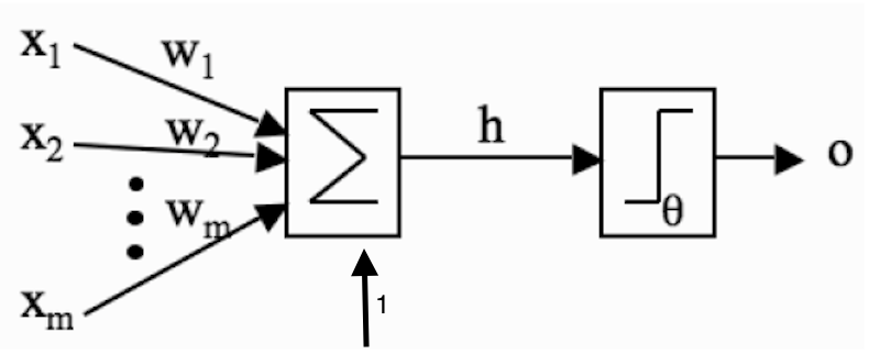 Figure 01. Basic Perceptron Model proposed by McCulloch and Pits.
The main characteristic of Perceptron is to have only one neuron. Basically, the model is composed by a set of inputs ( x1, x2, ..., xm ), weights ( w1, w2, .., wm ) and an activation function. The inputs represent the stimulus, the weights copy the strength of connections between neurons and the activation function imitates the property of neuron fire or not. All this elements together emulate a perceptron model which is nothing more than a mathematical operator that sums up all weights multiplied by inputs and the result is an input for activation function that provide a type of output as long as the result of the sum is greater than a threshold or other type of output, otherwise.
See, this is not that complicated model. I hope you are doing great so far, you can realize that neural network is nothing more than multiplications and sum whose result is applied to a function. And this is what really is.
Now, we need to map these stimulus in the inputs. Recall the example about eating delicious pizza in a new place. The stimulus was the taste of pizza and the tag was that the pizza was really good, so you learned that the pizza from that new place tastes good. Taste is not the only characteristic that make that pizza really good, in general, pizza has more observable features such as: size, format, smell, color, weight, consistency, temperature and so on, this set of features compose the concept of "good pizza" and this is exactly how we learning things from real world. Think about another example: How did you learn that a car is a car and not a truck? Probably when you were a little kid your parents pointed out a car and told you that it was a car and in other situation, they pointed a truck and told you that that big object was a truck. Indeed, what you did was observe few features that make these two objects different from each other and associate these observations with what your parents told you, for example, truck is bigger than car and may have many wheels, car does not have huge trunk and fits five people and so on. This is exactly what machine learning attempts to do: to teach algorithms how to classify objects providing dataset with examples of observable features where each observation has a tag or class.
The simple dataset
Alright, now that you know how the model and dataset should be for perceptron’s algorithm, it is time to code. Before we get fingers on fire, lets go to define which dataset and activation function we are going to use. We are focus on algorithm itself, so in order to keep the other variables as simple as possible, we are going to take a simple dataset originated from a well known OR logic function.
Starting with code, let’s store data in a R data frame format, like this:
data = data.frame( x1 = c( 0, 0, 1, 1 ),
                   x2 = c( 0, 1, 0, 1 ),
                   y =  c( 0, 1, 1, 1 ) )

print( data )
## x1 x2 y
## 1 0 0 0
## 2 0 1 1
## 3 1 0 1
## 4 1 1 1The dataset has only four observations which two of it belongs to class 0 and others to class 1. It is worth to see data in a graph. I am going to make a chart of it.
plot( data$x1, data$x2, type = 'n', main = 'Dataset OR', xlab = "x1", ylab = "x2" )
text( data$x1, data$x2, labels = data$y )
grid( nx = length( data$x1 ) + 1, ny = length( data$x1 ), col = 'black' )
The task here is to train a perceptron to perform a classification.
Let's do some training
First of all, what is training? Training has only one goal: find optimal values for weights that produce the minimum error when the algorithm performs a classification task. So, classification is simply to say if an determined input belongs to class 0 or class 1. To make it, the algorithm finds a hyperplane that separate these observations in two sides, one side supposed to has only observations from class 0 and other side has only examples from class 1. Things will be clear in the figure below:

Figure 02. OR classification
The parameters that define the hyperplane is given by the values of the weights. However, there is an infinite combination of it, each one define a different position of the hyperplane, there is certain positions that provoke misclassification. This error occurs when an input of a known class is classified by the algorithm as belonging to an different class. So, we need to choose the best position to avoid misclassification. Coming back to code, let’s initiate the values of weights randomly within a short range of values, like this:
weights = rnorm( mean = 0, sd = 0.1, n = ncol( data ) )

print( weights )
## [1] 0.07189541 -0.08588955 -0.12175474I took numbers randomly from normal distribution with mean equal zero and standard deviation equal 0.1. Wait a minute, so far we have seen two weights, one for each input, however the code above shows three weights. The third weights is for the bias inputs. Bias is a fixed input, generally either -1 or 1 that is responsible to activate a neuron even if the current inputs are both zeros. The last definition missing is the activation function. It will be the Heaviside step function as shown below:

Figure 03: Heaviside step function
The property of Heaviside step function is to have output equal 0 when the input is below a certain threshold and output 1 otherwise. You can already have the feel that the output of a activation function will be the guessing of the algorithm about what class the input belongs to. In this scenario, the Heaviside step function makes sense, because it allows us to compute the error in order to evaluate the perfomance of the classifier. Considering the value of the threshold equal 0.5, the activation function can be written as follows:
activation_function = function( net ){
                        if( net > 0.5 )
                            return( 1 )
                        return( 0 )
                    }
Now, we can finally write down the code for perceptron. Let’s take the first observation, add the bias values and multiply by the initial weights, the result will be put in activation function. After this, the value of error is computed and the weights are update in order to improve the assertiveness. To compute the error and update the weights, we are going to use the following expression where the parameter eta is the learning rate, this value define the step to walk throughtout the error function.
data = as.matrix( data )
net = c( data[1, 1:2 ], 1 ) %*% weights

y_hat = activation_function( net )

error = y_hat - data[1,3]

eta =  0.1

weights = weights - eta * ( error ) * c( data[ 1, 1:2 ], 1 )

print( weights )
## x1 x2
## 0.07189541 -0.08588955 -0.12175474This is the learning process with only the first observation, now we need to repeat it for the all examples available on the dataset. However, this loop needs to have a stop criterion which will define when the learning process should stop. To measure performance of the algorithm in classification task, we are observing the value of error, so it sounds reasonable to use it as a stop criterion, to be more precisely we are going to use the mean square error ( mse ) value. When the algorithm reaches a low values of mse, we will be satisfied with its performance. The code that performs the entire workflow training can be seen below:
perceptron = function( dataset, eta = 0.1, threshold = 1e-5 ){
                        data = as.matrix( dataset )
                        num.features = ncol( data ) - 1
                        target = ncol( data )

                        # Initial random  weights
                        weights = rnorm( mean = 0, sd = 0.1, n = ncol( data ) )

                        mse = threshold * 2
                        while( mse > threshold ){
                            mse = 0
                            for( i in 1:nrow( data ) ){
                                # Add bias and compute multiplications
                                net = c( data[ i, 1:num.features ], 1 ) %*% weights

                                # Activation function
                                y_hat = activation_function( net )

                                # Compute mse
                                error = ( y_hat - data[ i, target ] )
                                mse = mse + error^2
                                cat( paste( "Mean square error = ", mse, "\n" ) )

                                # Update weights
                                weights = weights - eta * error * c( data[i, 1:num.features ], 1 )
                            }
                        }
                        return( weights )
                    }
This function finds the optimal weights for perceptron model.
Look at that hyperplane!!
Alright guys, we reached the final part of this post. After we find the optimal weights for perceptron model, let’s take a look at the hyperplane. The function below charts the hyperplane over the input space.
shattering.plane = function( weights ){
                        X = seq( 0, 1, length = 100 )
                        data = outer( X, X, function( X, Y ){ cbind( X, Y, 1 ) %*% weights } )
                        id = which( data > 0.5 )
                        data[ id ] = 1
                        data[ -id ]= 0
                        filled.contour( data )
                    }
... Running the functions ...
weights = perceptron( data, eta=0.1, threshold=1e-5 )## Mean square error = 0
## Mean square error = 1
## Mean square error = 2
## Mean square error = 3
## Mean square error = 0
## Mean square error = 1
## Mean square error = 2
## Mean square error = 2
## Mean square error = 0
## Mean square error = 0
## Mean square error = 0
## Mean square error = 0shattering.plane( weights )
As you can see, the hyperplane separates the input space in two regions ( blue and pink ), each region represent that space where inputs are classified as belonging to class 0 and class 1. Also, you can observe that each time that you run the codes, you will get a different value of weights and consequently a change of the position of the hyperplane. For those who are still not familiar with R language, the complete perceptron code is store in my github repository, just copy and past it in a R console.
Good Conclusions and Future of Machine Learning
Perceptron is the first neural network model proposed, it works well on datasets that are linearly separable, for other types of datasets, perceptron presents many limitations that make it impossible to perform classification task with good results ( low error value ). For example, perceptron does not perform classification task over a dataset originated from logic function XOR. If you are curious person, you can run this code over a XOR dataset and see that perceptron is not able to separate class 0 and class 1, it will never reached a mean square error below to a given threshold. Also, try to classify a XOR dataset visually using a hyperplane. Are you able to draw a hyperplane that separate inputs from class 0 and class 1? Very likely not, you will fail miserably. I know that after all of this study, find a very limited classifier is frustrating. Do not be sad or desperate, this is not the end of machine learning, quite the opposite, it is just the beginning. Scientists figured out a way to surpass these limitations evolving the Perceptron algorithm to an algorithm called Multi-Layer Perceptron ( MLP ). Unlike perceptron, MLP is able to solve complex problems from simple logic function as XOR until face recognition. In the next posts, I am going to open up MLP black box implementing it from scratch and running it over a real dataset to show its power. Thanks for your time, you can check the complete code in github repository. Feedbacks are always welcome. See you guys soon.